Your guide to SimLab Desktop

Start here

SimLab Desktop User Manual • Version 0.1.25 • 24 October 2026

This manual follows a project from molecular inputs to docking, a solvated system, a short local simulation and analysis. It also explains the other tools and the optional Compute service. Use the numbered walkthrough in order for your first project; use the tool reference when you already know what you need.

Choose your route

Local route: create project → inspect and prepare → choose pocket → dock → build → export → Local Lab → analyse. Calculations run on your computer. Keep the app open and prevent sleep while work is running.

Optional remote route: build or import a prepared system → Compute → review stages → submit → monitor and retrieve results. This needs an online account, available resources and applicable credit. It is not required for the local tutorial.

What this edition covers

The instructions are checked against the 0.1.25 interface and recorded preparation, docking and build tests. The 181L practice protocol comes from the previously exercised book workflow. Screenshots illustrate the same workflow from the book’s 0.1.23-era interface; minor labels and results can differ. A new full simulation across every platform was not performed for this documentation edition.

The short trajectory is a training exercise, not evidence of convergence or biological activity. Use a protocol appropriate to your system for research. The book Beyond the Pose provides the scientific explanations behind these operations.

Files to download

Download simlab-desktop-practice.zip alongside this manual. Extract it fully. It contains the 181L protein, benzene input and reference, four teaching MDP files and a README. The manual PDF works offline; the web edition provides larger screenshots.

1. Install and activate

Use https://simlabscience.com/desktop/ and choose the installer for your operating system and processor. Leave space beyond the installer size for extraction, projects and trajectories. Back up projects before replacing an installed version.

macOS

Apple menu → About This Mac identifies your chip. Choose Apple Silicon for an M-series Mac, or Intel for an Intel Mac. Both published editions require macOS 14 or later. Open the DMG, drag SimLab Desktop to Applications, then launch the copy in Applications. Do not work from inside the mounted installer.

Windows

Settings → System → About → System type should show an x64-based processor and 64-bit Windows. The published installer supports Windows 10 version 1809 or later and Windows 11. No native Windows ARM or 32-bit installer is supplied. The 0.1.25 Windows installer is publisher-unsigned; verify its origin and checksum against the download page before deciding to run it.

Linux

Use the amd64 Debian package for Debian 12 / Ubuntu 24.04 or newer, or the x86_64 AppImage on a compatible system with glibc 2.36 or newer. For AppImage, enable execution in file properties, then open it. Follow the package manager’s installation prompts for the DEB. Verification instructions and signatures are linked on the download page.

First launch and updates

Connect to the internet for activation. Copy the activation licence offered on the download page, paste it in the app and choose Activate. Local tools can use cached entitlements; online services still need a connection. Open Help → Check for Updates to check the installed version. Never share private account credentials or retrieval tokens in screenshots.

2. Projects, inputs and the workspace

Choose File → New Project. Enter a meaningful name, choose Choose location & create… and select a writable local folder. For the tutorial use Manual - 181L benzene. Keep original files in a separate, unchanged folder.

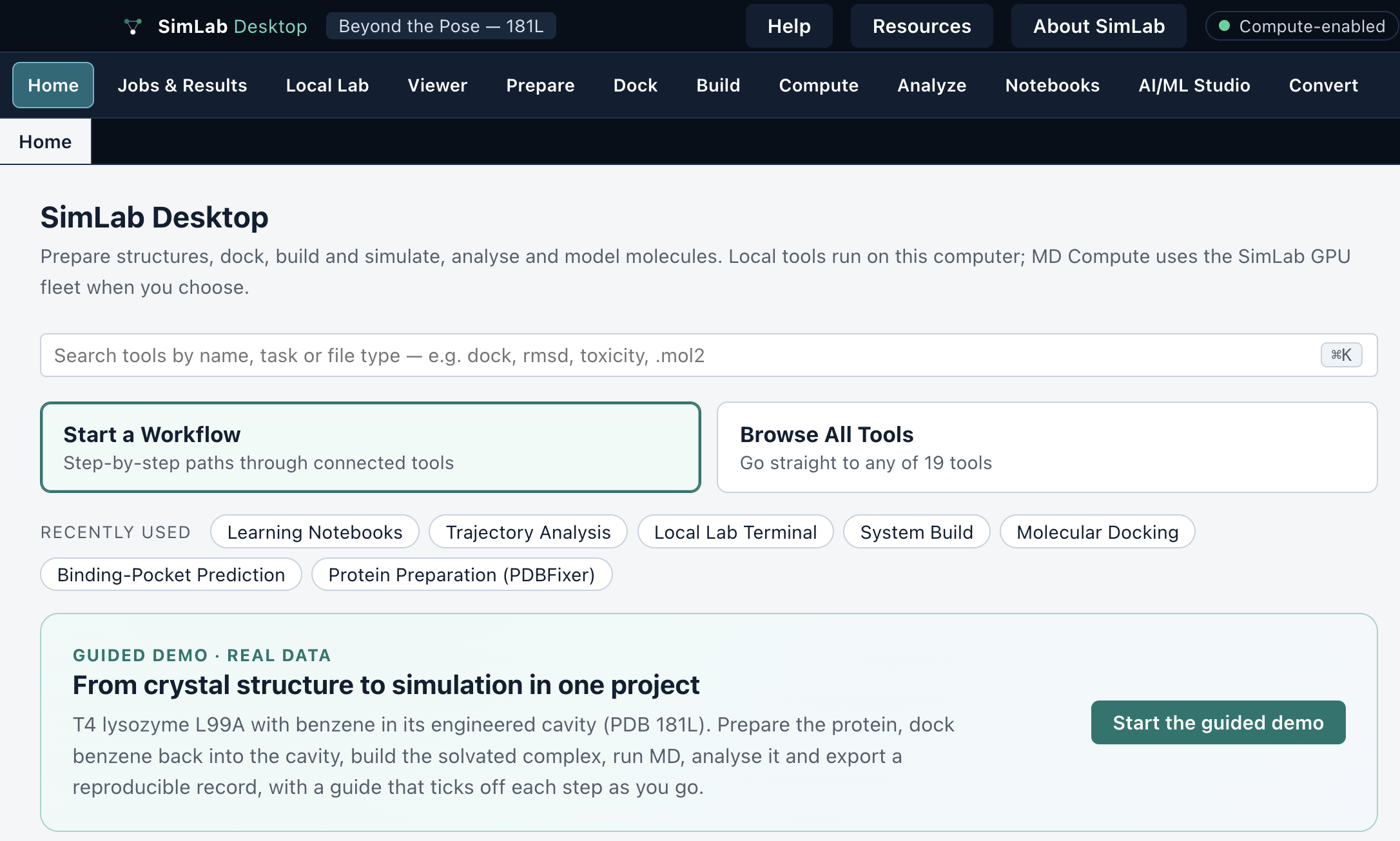
Import through the tool that needs the file: Dock → Upload receptor… for a receptor and Upload ligands… for ligands. General File → Import Files into Project can store an asset without the role needed by a tool. If a file is missing from a selector, import it through that tool instead of repeatedly copying it.

Jobs & Results and the Local runs panel show progress and logs. Runs can include other projects: check the project and run name before opening results. Use View controls or Focus workspace to reclaim screen space. Guided mode provides staged input; Advanced exposes more controls, not a different guarantee of correctness.

A SimLab project, an extracted build folder and a Local Lab working directory are different locations. The project stores app assets; the build ZIP stores simulation inputs; Local Lab runs commands in the directory you choose. Always check pwd and ls.

3. Inspect and prepare molecules

Before preparation, open the protein in Viewer. Check the intended chains, bound molecules, waters, missing regions and unusual residues. Decide what belongs in your model. Keep an unmodified structure for comparison.

Receptor preparation

Open Prepare / Receptor Preparation, select the receptor and inspect the proposed repair and removal choices. Run repair only when it is appropriate, inspect the output, then choose Use repaired receptor. Run preparation and choose Use prepared receptor for the downstream workflow. A repaired loop is a model, not experimental evidence.

In the 0.1.24/0.1.25 docking preparation path, incomplete residues can be excluded rather than rebuilt automatically. Read the preparation report: if an excluded residue is in the site you need, resolve that structural model before docking. Do not assume that pressing Prepare reconstructs every missing part.

Ligand preparation

Prefer SDF or MOL2 with defined connectivity and stereochemistry. Inspect charge, hydrogens and 3D coordinates. Coordinate-only PDB files can leave bond orders ambiguous. Use Molecule Studio for conformer/structure inspection and review the Dock preparation report. The separate Ligand Parameterization tool assigns MD force-field parameters; it is not a general docking-preparation wizard. A disconnected salt may be rejected; choose the chemically intended molecular species deliberately, rather than deleting fragments without understanding them.

For the practice project

The practice inputs already define a protein-only 181L receptor and benzene. Import inputs/181L_protein_only.pdb and inputs/benzene_crystal.sdf through Dock. Keep inputs/181L_benzene_reference.pdb separately. Do not repeatedly repair these inputs while comparing settings. Uploaded prepared PDBQT files are a separate route: 0.1.25 uses them as supplied, so their chemical preparation is your responsibility.

4. Predict a pocket

Open Dock → Binding-Pocket Detection. Select the same receptor you will dock against and choose Run locally. Wait for completion, then inspect the ranked pockets in the structure.

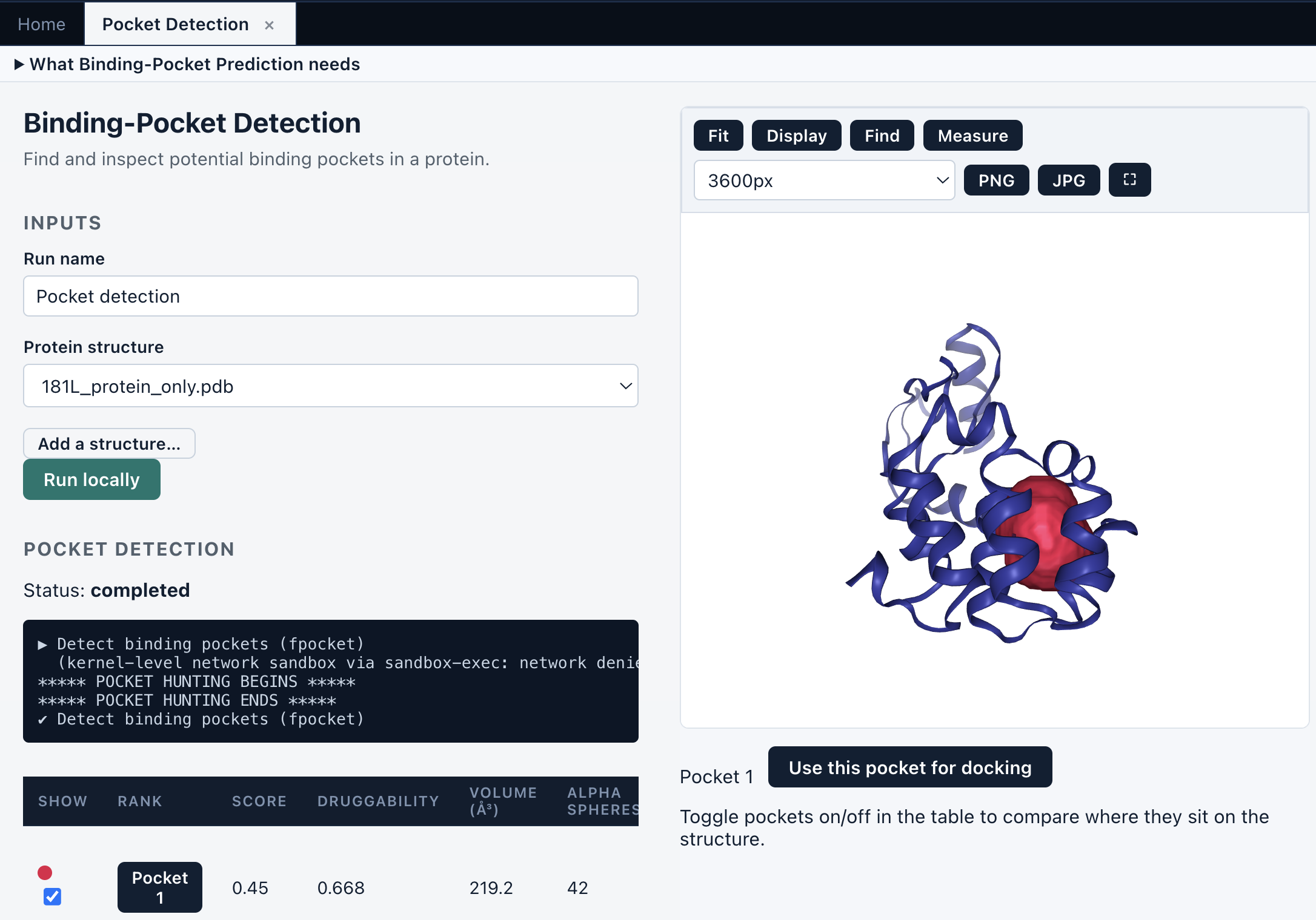
Select a candidate and choose Use this pocket for docking. Verify that the transferred receptor and search region are the intended ones. Predicted pockets are hypotheses; the top-ranked cavity is not automatically the correct biological site.

The docking form can automatically allow room for the largest prepared ligand when using a predicted pocket. The final shared box is recorded with results. This does not validate the site, account for every flexible conformation or prove that the ligand fits biologically.

Controlled practice settings

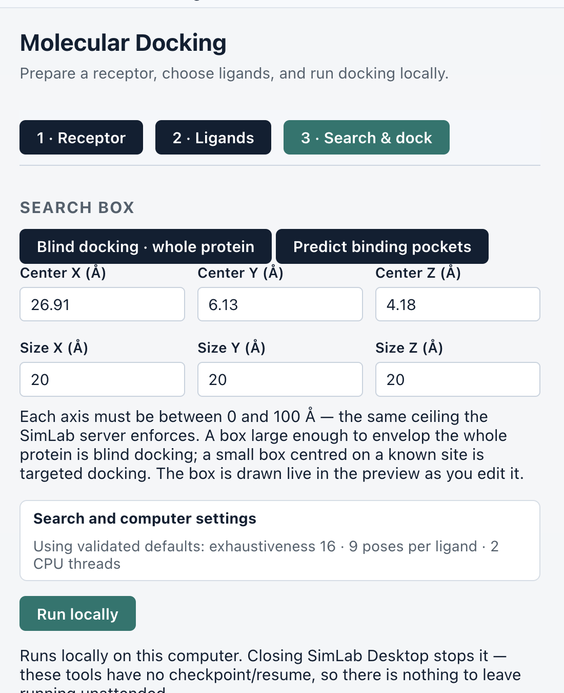
For this tutorial use a manual box: centre X 26.91, Y 6.13, Z 4.18 Å; sizes X 20, Y 20, Z 20 Å. If continuing from a pocket, turn off automatic sizing before entering these fixed values. Compare the cavity with the benzene reference. Keep all coordinates in the same receptor frame.

5. Dock and compare poses

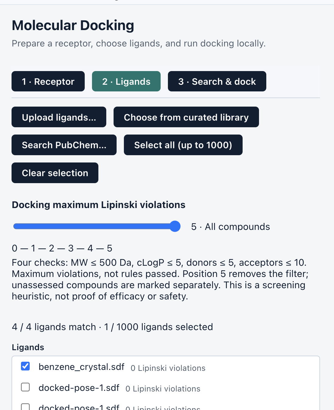
Open Dock. Select the 181L receptor in stage 1. In stage 2 choose benzene_crystal.sdf. Select only this ligand for the first exercise. The Lipinski filter is a screening aid; use the all-compounds setting if you need to see an unassessed imported ligand.

In Search & dock enter the fixed box from section 4. Set exhaustiveness to 16 and request 9 poses under Search and computer settings. Choose Run locally. Wait for the job to finish; use View log if it fails. Keep the app open.

Inspect several poses, not only the score. Check the ligand identity, cavity location and obvious clashes. Save the complete docking ZIP and record the selected pose number. Use Build selected complex → only after choosing a pose you can justify.

A completed job means the calculation ran, not that the pose is correct. A positive score is possible and should trigger inspection of the prepared receptor, ligand geometry and search region. Do not flip its sign or choose settings only to reproduce a desired negative number.

6. Make docking comparisons meaningful

For a command-line Vina comparison, use the exact prepared receptor and ligand PDBQT files exported by the job, the same box, Vina version, scoring function, exhaustiveness, pose count and seed from its log. Compare raw scores before rounded spreadsheet values.

Uploaded PDBQT files remain unchanged in 0.1.25. A failed ligand is reported separately; do not silently count it as a zero-score result. Preserve the seed, engine version and preparation report with the scores.

Previous release testing matched the command-line run for 19 completed ligands in a 20-ligand comparison; the disconnected salt was a separate failure. That is evidence for those matched inputs, not a promise that any two independently prepared projects agree. Small processor-dependent differences were observed; a repeat on the same tested platform reproduced its own scores.

PyRx and SimLab can prepare different chemical inputs even when both call Vina. Hydrogens, protonation, atom typing, connectivity, retained waters, receptor treatment and the box all matter. Vina uses hydrogens to identify donor types; adding hydrogens is not a universal adjustment that makes scores more negative or more correct.

Reference: https://autodock-vina.readthedocs.io/en/latest/faq.html. For the practice exercise, compare pose geometry with the reference; do not use an old screenshot score as a pass/fail threshold.

7. Build the selected complex

From the selected docking pose choose Build selected complex →. Confirm the transferred protein and ligand, including the pose number. Review the ligand net charge. Benzene is neutral (0).

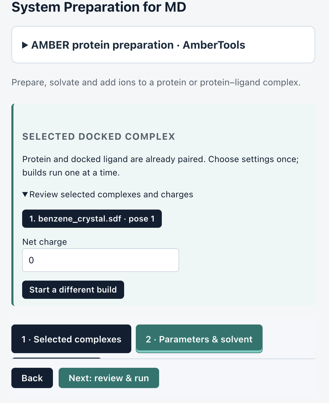
For this practice protocol choose AMBER14SB / GAFF2, TIP3P water, cubic box, 1.2 nm padding and 0 M added salt, retaining neutralization. These are teaching settings, not universal defaults. Do not substitute CHARMM or OPC while using this practice MDP set.

For your own system use a compatible family: for example AMBER ff19SB with its offered OPC route, or the offered CHARMM36m route with its compatible ligand and water parameters. Do not combine files from different force fields to satisfy a missing-include message. Arbitrary ligands need parameterization; GROMACS does not infer those parameters by itself.

Choose Next: review & run, inspect the summary and choose Build locally. Read the completed build report and inspect the resulting solvated structure. The builder prepares a starting system. Files named minimization or equilibration do not mean those simulations have completed.

Standard automatic complex building is for a protein plus a small-molecule ligand. Metals, covalent ligands and specialized cofactors can need a supplied parameterized model; see the additional-tool reference.

8. Export a complete, portable system

Choose Download build ZIP and extract it completely into a new writable folder. Open its run/ subfolder. Read the exported README before choosing inputs. Preserve the entire folder tree.

Files and their jobs

step3_input.gro: built starting coordinates, atom order and box. topol.top: top-level topology. toppar/ and force-field folders: included parameters. index.ndx: named atom groups. *.mdp: proposed simulation settings. A topology may include files outside toppar/ within the exported tree; keep all referenced files.

A CHARMM-GUI export and a SimLab export need not list the same filenames in toppar/. A .prm can contain an included parameter definition; a .str is not automatically a runnable GROMACS topology. What matters is the complete include tree, compatible definitions and successful preprocessing. Do not rename extensions or copy a different project’s topology to make the lists match.

Prepare for Local Lab

Copy em.mdp, nvt.mdp, npt.mdp and md-validation.mdp from the practice kit’s mdp/ folder into a fresh copy of your extracted run/ folder. Keep the original export unchanged. These practice files are for the stated 181L/benzene AMBER14SB/TIP3P exercise, not generic CHARMM settings.

Before running, you should see step3_input.gro, topol.top and all included files alongside those four MDP files. Do not use a temporary intermediate coordinate file or work inside the ZIP preview.

9. Open Local Lab in the right directory

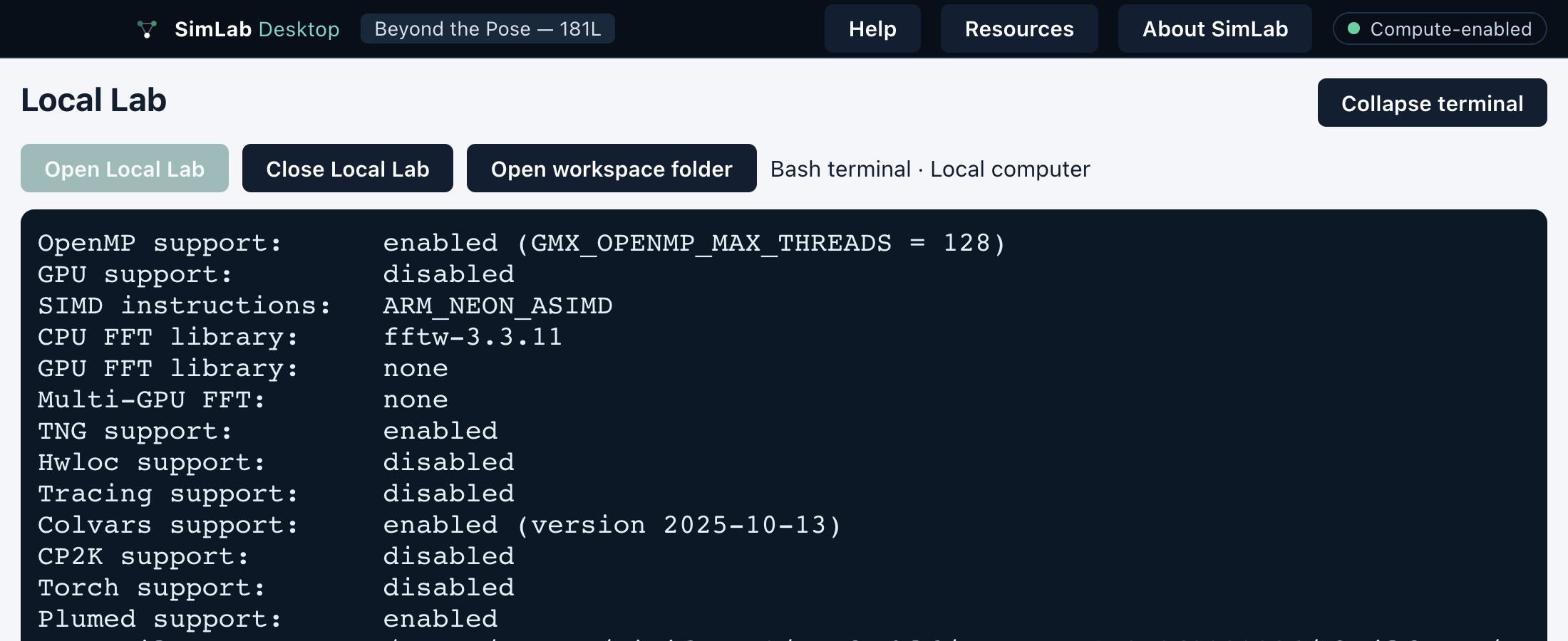
Open Local Lab → Open Local Lab. Select the extracted working run/ folder and confirm opening the local terminal. Wait for the Bash prompt. Expand terminal for more space. This is Bash on Windows too; PowerShell commands do not belong at this prompt.

pwd
ls
gmx --version
export OMP_NUM_THREADS=4

pwd must show your chosen working folder. ls should list the files from section 8. Record the GROMACS version. The example uses four OpenMP threads; if choosing another count, use the same value in OMP_NUM_THREADS and every -ntomp argument.

Use quotation marks around paths containing spaces. Open workspace folder reveals the files in your file browser. nano and vi edit plain-text files; save before launching a calculation. Keep this terminal open during local runs. Ctrl+C interrupts a foreground command; Close Local Lab can stop the calculation.

cd "path/to/your/run"
ls -l topol.top step3_input.gro

The cd path above is a placeholder: replace it with your actual Bash path, or simply choose the correct folder when opening Local Lab. Windows paths should use the form shown by the Bash terminal, not an unquoted Windows Explorer path.

10. Minimize and inspect

Run these commands in the folder established in section 9. The MDP files must be the practice files copied in section 8. Run the second command only if preprocessing succeeds.

gmx grompp -f em.mdp -c step3_input.gro \
  -p topol.top -o em.tpr -maxwarn 0
gmx mdrun -deffnm em -ntmpi 1 -ntomp 4

grompp combines settings, topology and coordinates into em.tpr. mdrun performs the calculation and writes em.gro, em.log and em.edr, among other outputs. Read the final stopping reason and compare the maximum force to emtol in em.mdp.

tail -n 40 em.log
gmx energy -f em.edr -o potential.xvg

In the energy menu select Potential by its displayed name or current menu number, then finish the selection as prompted. Inspect the energy trace and geometry. A negative potential energy alone does not prove minimization succeeded.

If preprocessing stops

Read the warning or error above the final fatal-error message. Resolve missing includes, coordinate/topology disagreement or geometry problems. Do not add a blanket -maxwarn allowance to force a run through. An excluded-pair distance warning needs investigation of connectivity and geometry; an upload timeout is a different kind of failure.

Reference: https://manual.gromacs.org/current/user-guide/run-time-errors.html. Preserve the input set and log when asking for help.

11. Equilibrate: NVT then NPT

Continue only after reviewing minimization. This tutorial uses 20 ps NVT and 50 ps NPT to demonstrate the mechanics; research equilibration may require much longer.

NVT

gmx grompp -f nvt.mdp -c em.gro -r em.gro \
  -p topol.top -o nvt.tpr -maxwarn 0
gmx mdrun -deffnm nvt -ntmpi 1 -ntomp 4
gmx energy -f nvt.edr -o temperature.xvg

Select Temperature in the energy menu. Check the log for constraint or numerical problems and inspect the temperature trace. Preserve nvt.gro and nvt.cpt.

NPT

gmx grompp -f npt.mdp -c nvt.gro -r nvt.gro \
  -t nvt.cpt -p topol.top -o npt.tpr -maxwarn 0
gmx mdrun -deffnm npt -ntmpi 1 -ntomp 4
gmx energy -f npt.edr -o density.xvg

Select Density. Inspect pressure, volume/box behavior, energy and structure as well. A plausible final density does not establish a stable distribution. If there is persistent drift or instability, investigate and extend an appropriate equilibration protocol before research production.

Do not substitute coordinates or checkpoints from another run. -r supplies reference coordinates for restraints; -t transfers checkpoint state where the MDP requests continuation. Preserve both the files and the settings.

12. Generate a teaching trajectory

For learning the final stage and analysis tools, the supplied md-validation.mdp produces 100 ps. Treat it as a pipeline demonstration, not a claim that the short equilibration above has established a research-ready ensemble.

gmx grompp -f md-validation.mdp -c npt.gro \
  -t npt.cpt -p topol.top -o md-validation.tpr \
  -maxwarn 0
gmx mdrun -deffnm md-validation -ntmpi 1 -ntomp 4
gmx check -f md-validation.xtc

Keep md-validation.tpr, .xtc, .gro, .edr, .log and .cpt together. Check the recorded final step/time and warnings. The XTC contains saved coordinates; the EDR contains recorded energy terms. Neither replaces the topology or run-input file.

Interruptions and continuation

Do not start a second copy while the first is still running. For a compatible interrupted run, retain the original output files and checkpoint and resume from the same directory:

gmx mdrun -deffnm md-validation \
  -cpi md-validation.cpt -ntmpi 1 -ntomp 4

This resumes an interrupted run; it does not extend a completed TPR beyond its planned duration. Research extensions need a deliberate new run-input duration and matching checkpoint handling. Preserve backups before changing run plans.

13. Analyse and export

Open Analyze / Trajectory Analysis. Import the matching md-validation.tpr and md-validation.xtc; add md-validation.edr for energy analyses when requested. Select RMSD, RMSF or radius of gyration and review the atom selections. Choose Run locally and inspect plots and logs.

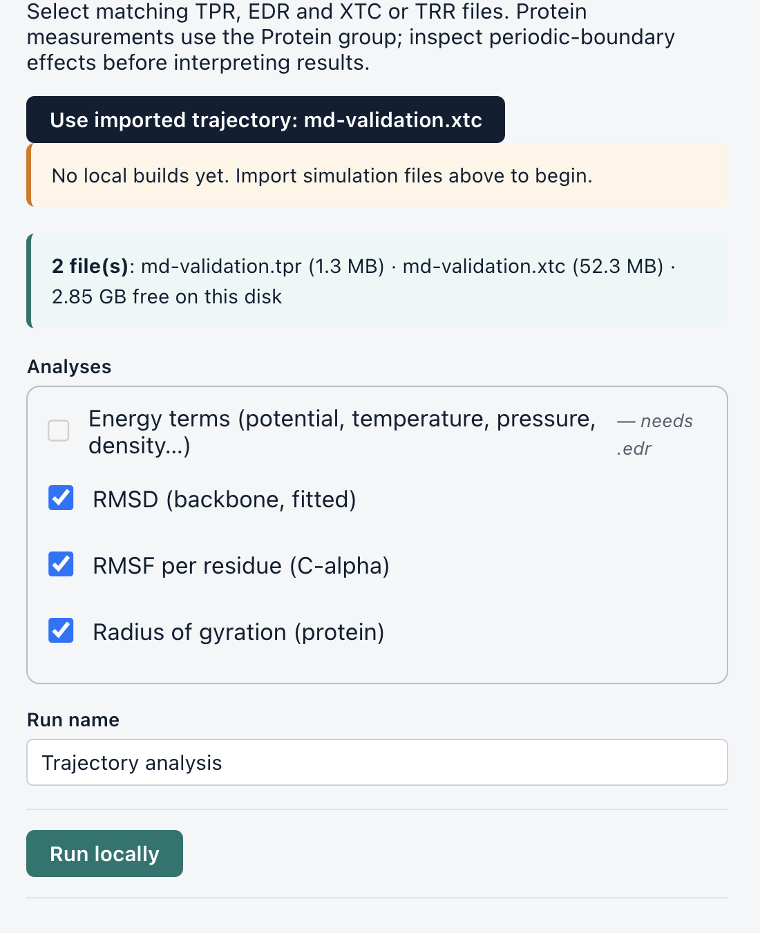
Check periodic-boundary handling and alignment before interpreting motion. Atom count alone does not prove that a structure matches a trajectory: atom order must also match. Document the fitting group, measurement group, time window and units.

For visual playback, open the matching GRO in Viewer and choose Load XTC / TRR. The documented viewer limit is 128 MB. Make a deliberate reduced/processed copy if needed, keeping the full original trajectory. Viewer playback does not automatically reconstruct periodic molecules or align frames.

Export numerical results alongside figures. A useful report says what was measured, over which interval, with which selections, and what remains uncertain. A 100 ps exercise does not establish ligand residence time, converged binding energy or clinical activity.

A complete practice archive

Keep original inputs, preparation report, docking configuration and poses, selected pose identity, complete build export, MDP files, command history, logs, checkpoints, trajectory, numerical analyses and a short interpretation. Someone else should be able to follow your decisions without guessing.

14. Compute: an optional separate route

Compute runs remote jobs and can incur charges. It is not needed for the Local Lab exercise. Sign in using your own account and review the current rates and balance before submitting.

From a completed build choose Simulate this system on SimLab compute → or open Compute and select System built in this project. For an external system choose Choose a prepared system folder… and select the fully extracted folder containing coordinates, topology, includes and MDP files.

Review the selected coordinate/topology and stage order. Inspect each MDP, including any fallback template. For external protocols preserve all intended equilibration stages rather than replacing them with a single default. Resolve missing includes before submitting.

Submit once and monitor the log: project creation, file upload, preprocessing and running are different stages. A created project does not mean files uploaded. A queued job is not a completed simulation. Already submitted remote jobs may continue if you close the app; this release can require the app to stay open to advance later stages, or continuation from the website Compute workspace.

Known 0.1.25 upload limitation

A slow upload can stop with “SimLab Compute did not respond in time,” sometimes while uploading step3_input.gro. This can be a transport deadline, not a topology or molecular-geometry failure. The longer-upload fix was not part of published 0.1.25 at this manual’s date. Check the remote project state before retrying to avoid duplicate projects or submissions. Preserve the project identifier and log; use Local Lab for local work when appropriate.

Do not repeatedly rebuild the molecule or raise maxwarn to solve a network timeout. If a current-project selection still requests files, verify the selected build completed and that its exported files remain available. Import the complete export as an alternative, preserving the directory structure.

15. Find every tool

Home → Browse All Tools lists the scientific tools. Press Ctrl+K on Windows/Linux or Cmd+K on macOS, outside the terminal, and search by tool name, task or file type. Use arrow keys and Enter to open a tool; Escape closes the launcher. Inside Local Lab, terminal shortcuts retain their shell meaning.

The app catalogue contains 19 scientific tools. The earlier walkthrough covers Protein Preparation, Binding-Pocket Prediction, Molecular Docking, System Build, Local Lab Terminal, Trajectory Analysis and MD Compute. The sections below complete the reference for every remaining tool and the AMBER subpanels.

A tool can require an open project even when its input files exist on disk. Create/open a project first if prompted. Local jobs appear in Local runs; AI/ML also has its own Runs & results tab. Remote jobs use their service status.

Choose the task before the format

Docking preparation creates docking inputs. Ligand Parameterization assigns MD parameters. Converter changes representation. These are distinct operations: converting a PDB to PDBQT does not validate chemistry, and an AMBER parameterization does not create CHARMM parameters.

The reference documents the installed 0.1.25 controls and expected output types. It does not claim that every optional scientific method has been rerun for this manual. Use the complete example first, then validate additional methods for the intended inputs.

16. Molecular Viewer: inspect, edit and export

Open Molecular Viewer from Home or the launcher. It can work without a project. Load a supported structure such as PDB, mmCIF, GRO, SDF, MOL2, PDBQT or XYZ, then choose the active structure/model.

Display and selections

Expand Display to choose cartoon, licorice, lines, surface, ball-and-stick or spacefill. Set colouring/background and show or hide waters and ions. Use sequence/residue search to select a region, then focus it. Expand the viewer when labels are crowded.

Find offers contact searches including polar contacts, salt bridges, hydrophobic contacts and metal coordination. Searches act within the active structure; load the combined complex to inspect protein–ligand contacts. Geometric candidates are not experimentally proven interactions.

Edits and outputs

Residue deletion and standard amino-acid mutation create an edited copy. Inspect the result and use Undo for an unwanted edit. An edited structure still needs chemically appropriate preparation before calculations. Save As lets you choose the current model/frame, selected residues or visible atoms, then a supported coordinate format. PNG/JPG saves a picture, not coordinates.

For XTC/TRR playback load matching GRO coordinates, then Load XTC / TRR. Match both atom count and order. The documented trajectory size limit is 128 MB. Play, pause, scrub and export the selected frame. Periodic reconstruction and alignment must be handled deliberately before interpreting motion.

17. Protein–Ligand Interactions

Open Interactions from a docking result or the launcher with a project open. Supply a combined protein–ligand complex, or use the selected docking pose. Verify the ligand identity and pose number before analysis.

Run and inspect

Choose the ligand whose surroundings you want to analyse. Run the interaction analysis, then compare the residue/contact table and 2D view with the 3D geometry. Check that ligand atoms, residue names and distances refer to the intended complex.

Inspect hydrogen bonds, hydrophobic contacts, salt bridges and other reported classes in chemical context. Missing hydrogens, ambiguous bond orders and protonation can change the assignments. Do not count every line in a figure as an independent stabilizing interaction.

Export and next step

Export the available diagram as PNG/JPG at a readable resolution, and retain the associated numerical report/log through the run files or ZIP. Record which pose was analysed. A static pose contact map does not report contact persistence across a trajectory.

If no contacts appear, confirm that receptor and ligand occupy the same coordinate frame and belong to the same loaded complex. Do not move the ligand arbitrarily just to create contacts.

18. Compound Library and PubChem

Open Curated Compound Library. Browse categories, search compound names/identifiers and inspect the displayed properties. Browsing the bundled library is local; adding selections to a scientific workflow requires the appropriate project.

Select a set

Maximum Lipinski violations filters on molecular weight, cLogP, hydrogen-bond donors and acceptors. Settings 0–4 retain compounds at or below that count; setting 5 removes the filter and includes unassessed compounds. If an uploaded compound seems to vanish, check this filter.

Project ligands accepts your own library; multi-record SDF files are split into individual ligands. Review the resulting names and counts before selecting a batch. Docking supports up to 1,000 selected ligands per run; a large run can take substantial local time.

Fetch and transfer

Use the PubChem search to look up a name or CID online, inspect the result and import a copy into the project. Confirm whether coordinates are 2D or 3D and inspect stereochemistry/protonation. Send the intended selected compounds to Docking or the available property tools.

Keep measured values separate from calculated descriptors and predicted endpoints. Lipinski filtering is not proof of oral activity or safety. Save source identifiers and the exact selected molecular structures with screening results.

19. Molecule Studio

Open Molecule Studio to draw/import molecules, organise a collection and calculate RDKit properties. Enter a chemically valid structure or import supported SDF, MOL, SMI or CSV files. A CSV can provide SMILES and a name column. The import workflow accepts up to 200 molecules per file.

Prepare and inspect a molecule

Calculate descriptors and generate a 3D conformer using the offered MMFF94/UFF route. Inspect connectivity, charge and stereochemistry in the displayed molecule. A generated conformer is a starting geometry, not the experimentally bound state.

Search and chemical space

Use similarity search to compare with a query and substructure search for a defined fragment. Chemical space provides PCA/t-SNE and clustering on the available standardized descriptors. Select a plot point to inspect its molecule. Proximity in a projection is not a measured similarity in biological activity.

Export and hand off

Export the displayed results as CSV, SDF or SMI, or export Morgan fingerprints where offered. Use the available transfer controls to send selected molecules to ADMET, Docking or AI/ML. Use in DFT transfers generated 3D geometry to the quantum panel; review charge and multiplicity there.

A simple interface exercise is to enter ethanol (CCO), calculate properties, generate a conformer and export SDF. Check that the exported structure is the same intended molecule. This is a file-handling exercise, not a docking or ADMET validation dataset.

20. Molecule Converter

Open Convert / Molecule Converter. No account or project is required in the installed converter panel. Add files… and select files sharing the same input format. The originals remain unchanged.

Choose the conversion

Choose From and To using the format selectors; Find a format filters the available formats. The actual readable/writable formats are detected from the installed engine. Select One output per input file, Combine records into one file, or Separate file for each molecular record.

Merge supports SDF, SMI, MOL2 and XYZ. Split is useful when the destination represents a single molecule. Choose a format that can retain the data you need; PDB/XYZ and other simple formats can lose bond orders, charges, stereochemistry or multiple records.

Run and recover files

Choose Convert files. Inspect the completion status and View log. Open converted files reveals the output directory; Download converted files ZIP saves a portable copy. Cancel interrupts an active conversion.

The converter does not optimize a molecule or create scientifically validated parameters. Reopen representative outputs and verify record count and chemistry. Do not use conversion as a substitute for ligand parameterization or receptor preparation.

21. Ligand Parameterization: GAFF2 / AM1-BCC

Open Ligand Parameterization with a project containing the intended ligand. This standalone route generates AMBER-compatible small-molecule parameters locally. It is different from preparing PDBQT for Vina.

Inputs and controls

Select Ligand / cofactor structure, set Net molecular charge to the intended integer charge and enter the Residue name. Inspect the preview before running. Use a chemically defined ligand with reliable bond orders and stereochemistry; an inferred PDB bond pattern can be wrong.

Run and read the outputs

Run the parameterization and monitor Local runs. The pipeline uses antechamber for GAFF2 atom typing and AM1-BCC charges, parmchk2 for a parameter-coverage check and tleap for an AMBER topology. Review the typed MOL2, coverage report, topology and logs in the completed results. Preserve the full output set through the run files/ZIP.

Parameter assignment does not prove those parameters are suitable for your scientific question. If antechamber fails, inspect chemistry, net charge and its full error rather than changing charge until it runs.

Where these parameters belong

Use the output within a compatible AMBER-family workflow. It is not a CHARMM/CGenFF parameter generator. Metals, covalent attachment, unusual cofactors and unsupported chemistry need an explicitly validated model. A form label mentioning cofactors is not a promise of general metal-centre parameterization.

22. ADMET Prediction

Open ADMET Prediction with a project. Enter the intended molecule as SMILES in the panel, or transfer a molecule from Studio/library through an available control. Give the run a recognizable name.

Run and interpret

Run the local prediction and monitor Local runs. Review the grouped predicted endpoints alongside physicochemical descriptors and drug-likeness flags. Preserve the input SMILES with the output, so you know exactly which chemical species was evaluated.

Read endpoint labels, units and whether a result is a value or a probability. Predictions are model estimates, not experimental pharmacokinetics, toxicity measurements or clinical safety conclusions. An unusual molecular class may be outside the model’s reliable domain.

Export and compare

Retain the result table and log using the available result/run export controls. For comparisons, use the same input-preparation policy and model version across the set. AI/ML Studio can import available batch ADMET results, but imported predictions must remain labelled as predictions rather than experimental training labels.

If a structure cannot be parsed, correct the chemistry/source data. For salts or mixtures decide the intended molecular species explicitly and record that decision; do not treat silent fragment removal as a scientific validation.

23. Protein–Protein / Peptide Docking

Open Protein–Protein / Peptide Docking (LightDock) with a project. Select separate receptor and binding-partner PDB structures. This is not the small-molecule AutoDock Vina panel.

Prepare and configure

Inspect both partners for missing atoms/side chains and the intended biological assembly. Review Swarms, Glowworms per swarm and Simulation steps. Use residue restraints only when you have a defensible basis and the offered restraint syntax is satisfied.

Run and inspect

Start the local run and monitor the log. Inspect ranked complexes and available clustering, including clashes, interface geometry and whether a restraint drove an implausible result. Preserve the settings and both original partner structures.

Outputs and limitations

Export ranked complexes and the run record from the result controls. LightDock scores are not Vina affinities and should not be compared numerically to a small-molecule docking score. A high rank does not prove a biological interaction.

Do not feed a peptide into the small-molecule workflow merely to avoid a failed protein–protein setup. Choose the method appropriate to the size, flexibility and question, then validate against known interfaces where possible.

24. MM/GBSA Binding Energy

Open MM/GBSA with a project and choose Import a folder… for a complete GROMACS analysis folder. It needs a matching TPR, XTC/TRR trajectory, NDX index, TOP topology and every topology include, such as toppar/. Inspect the detected filenames.

Groups and sampling

Enter Receptor group and Ligand group exactly as defined in the index. Check atom membership; the groups should represent the intended partners. Choose the Generalized Born model and Start frame (1-based); leave End frame blank only if you intend to use the final available frame.

Run and review

Resolve displayed input issues, then start the local calculation. Many frames can take substantial time. Inspect the log, reported binding estimate and per-term breakdown. Preserve settings, frame interval/selection, topology and raw outputs with the result.

Interpretation

Confirm force-field compatibility and how solvent/ions are handled. Do not replace an incompatible topology with one from another system. An endpoint estimate is sensitive to the model and sampling; a short demonstration is not a converged affinity calculation.

Use the same protocol when comparing systems and assess uncertainty from adequate sampling. Do not present an automatically generated negative number as proof of binding or compare it directly with a Vina score as though they were the same quantity.

25. AMBER protein preparation

Open Build and expand AMBER protein preparation · AmberTools. This is a separate protein-only AMBER-output route, not the main GROMACS complex builder.

Inputs

Choose protein PDB for a prepared standard-residue protein. Check protonation, missing regions and disulfides first. Select the offered protein force field (ff19SB or ff14SB), water model, water-box padding in Å and NaCl concentration after neutralization. Do not confuse this padding unit with the nm setting in System Build.

Run and inspect

Choose Prepare AMBER system. Monitor the status, View log and Open run folder. A successful run supplies PRMTOP, INPCRD, solvated PDB and an ion verification report. Use Export run ZIP to retain the complete set.

This installed preparation form does not run minimization. Minimize and equilibrate using an appropriate AMBER protocol before production. Its filenames are not interchangeable with the GROMACS tutorial filenames.

Scope

Ligands, metals and nonstandard residues require their own compatible parameters and are not supported by this protein-only form. For a preparameterized complex use the separate supplied-topology build route described in the troubleshooting section. Do not discard a necessary cofactor simply to satisfy the form.

26. AMBER trajectory analysis: CPPTRAJ

Open Analyze and expand AMBER trajectories · CPPTRAJ. Choose topology (PRMTOP/PARM7) and Add trajectories… for matching NetCDF or MDCRD files with identical atom order.

Order and time

Arrange files chronologically with Move up and remove unwanted files. Remove duplicated boundary frames before import. Enter the actual Time between saved trajectory frames (ps); the plot’s time starts at zero using that interval. All input files must share the interval.

Use Sample every N frames deliberately. For multiple files use stride 1, or combine them externally before subsampling. The default atom mask @CA selects protein alpha carbons. RMSD aligns to the first sampled frame, RMSF uses that alignment and Rg uses the selected atoms.

Periodic imaging

Autoimage requires periodic box information. CPPTRAJ uses the first molecule as its default anchor; inspect the result for multimers, membranes or other nonstandard assemblies. Prepare such trajectories separately when that default is inappropriate.

Run and outputs

Choose Analyze AMBER trajectory. Review sampled frame count, RMSD, RMSF and radius-of-gyration plots, plus the log. These AMBER plots use Å for distances; do not silently compare them to GROMACS nm values. Open run folder or Export run ZIP to preserve tables, input script and log.

27. DFT / Quantum Chemistry

Open DFT / Quantum Chemistry with a project. This panel edits inputs locally and submits calculations to the online fleet. It does not provide an offline quantum-computation runner.

Geometry and model

Choose Import XYZ, or transfer generated 3D geometry with Use in DFT from Molecule Studio. Load H₂ example is available for an input-editing exercise; loading it does not require submitting a job. Check the coordinates, net charge and spin multiplicity.

Choose the offered engine (PSI4, ORCA or XTB), calculation type, method/basis and applicable solvent/settings. Available fields depend on the engine. XTB is a distinct approximate quantum method, not a DFT functional merely because it shares this panel. Review the generated input and any engine-licensing acknowledgement.

Submit only after review

Review the estimate, account/access requirements and requested resources, then submit deliberately. Preserve the returned public code and retrieval token securely. Do not put private retrieval tokens into a public report or screenshot.

Results

Use Jobs to inspect status and engine logs. A queued job is not finished. Preview/download the available output files and review convergence, charge/spin and the requested calculation’s completion. A downloaded output file alone does not establish a converged electronic or optimized geometry result.

28. AI/ML Studio: Data, Curate, Explore and Profile

Open AI/ML Studio with a project. The installed suite has Data, Curate, Explore, Profile, Train, Runs & results, Screen and Models tabs. Computation runs locally; resource availability depends on the machine and installed runtime.

Data

Choose Import molecules… for CSV, TSV, SMI, SDF, MOL or MOL2 (up to 200 MB in the panel). Use Example: ESOL solubility or Example: BBBP permeability for practice. Inspect the table and identify the SMILES, name and target columns. Imports are fixed snapshots with checksums.

Import from elsewhere in SimLab can bring in Molecule Studio, library compounds, batch ADMET predictions or docking results. Preserve the meaning and units of the target: a model trained on docking scores predicts those scores, not measured biological activity.

Curate

Select the dataset and SMILES column, review the offered standardization/filter choices and run curation. Inspect removed rows and Standardization changes in Runs & results. Keep the original dataset; use the resulting curated dataset deliberately for later steps. Check duplicate structures and inconsistent labels before training.

Explore and Profile

Explore selects molecular features and projections such as PCA, t-SNE or UMAP, with optional clustering and advanced settings. Record the random seed and chosen representation. Profile provides property/rule checks, similarity search and diverse-subset selection. Inspect the returned molecules; attractive clusters or alert flags are not evidence of activity.

29. AI/ML Studio: train and evaluate

In Train choose the dataset, SMILES column, target and task. Use Regression for a continuous endpoint or Classification for classes; specify the positive class when relevant. Check units, missing labels and whether classes are meaningful.

Features and models

Select fingerprints/descriptors or the representation supported by the chosen model. Classical choices include random forest, extra trees, boosting, SVM, nearest neighbours and appropriate linear/classification models. Neural choices include MLP, graph models and SMILES models. Options shown by the interface still depend on runtime availability and input suitability.

Set training/device options and a reproducible seed. Auto can use an available NVIDIA or Apple GPU, otherwise CPU. Use a small baseline before selecting many models or expensive deep-learning settings. Transfer learning needs a compatible saved model and a deliberate fine-tuning choice.

Splits and validation

Choose a split strategy matching the research question: scaffold, similarity clusters, random, stratified, group or time where supported. Review the train/validation/test sizes and grouping/time column. Keep related or duplicate compounds from creating an artificially easy test. A scaffold split is useful but not universally sufficient.

Run training and inspect Runs & results: validation comparison, selected model, held-out test metrics, split/leakage audit, applicability-domain information and available explanation plots. Regression and classification metrics answer different questions. Review probability calibration or conformal settings where used; nominal intervals are not a guarantee on out-of-domain chemistry.

Do not repeatedly tune against the reported test set. Record the dataset checksum, split, seed, settings and software versions. A high training score or a plausible heatmap alone does not validate a predictive model.

30. AI/ML Studio: screen, export and reuse

After training, open Screen and select the saved Model. Choose a molecule file (CSV, SMI or SDF) or a dataset in the project. The panel supports libraries up to 250,000 molecules, but available memory and runtime still constrain practical jobs.

Inspect predictions

Run screening and review results with uncertainty/applicability flags. Use Minimum train similarity and Maximum uncertainty filters deliberately. Review molecular identities and ranking direction; a larger predicted value is not always preferable for the endpoint.

Select hits and send them to Molecule Studio, ADMET or Docking using the available controls. Combining results with an ADMET or docking run adds comparison columns; it does not convert predictions into experimental evidence. Preserve the screening input and rejected/failed records.

Models and portable records

Models lists saved model packages and their target/test performance. Report opens the training record; Screen reuses a model; External test… evaluates a separate dataset. Export saves the model package; Import model package… loads one for supported reuse.

Respect the displayed trust status. Pickle-based estimators from elsewhere can require Rebuild rather than direct loading. Do not bypass that restriction. A rebuild can produce different results across software/hardware; keep provenance and compare the resulting evaluation.

Practical first exercise

Use the bundled ESOL example, inspect its endpoint, curate a copy, train a modest classical baseline with a recorded split/seed, then inspect the test and leakage reports and export its package. The purpose is to learn the controls; it does not validate a new drug-discovery model.

31. Learning Notebooks

Open Learning Notebooks. Choose Open in Local Lab workspace to reuse that folder, or Choose a folder… for the files you want to analyse. The notebook server and kernels run on your own computer; the browser connects to a local address.

Open and run a notebook

When the session is ready, choose Open in browser. Open analysis_template.ipynb in the notebook file list. Read its compatibility notes, edit file paths for your actual system and run cells in order with Shift+Enter. Python cells are not plain Bash terminal prompts.

The template covers RMSD, RMSF, radius of gyration and hydrogen bonds. Method A reads GROMACS-generated XVG data; Method B works directly with trajectories through MDAnalysis. Choose the method intentionally and verify atom selections, periodic treatment, alignment and units.

Save and stop

Save the notebook, figures and data together. Check status refreshes session state. Stop notebook session ends running kernels, so save and finish work first. Saved notebooks remain in the workspace. Keep SimLab Desktop open while using its notebook session.

Teaching templates are installed in a versioned folder; existing nonempty notebooks are preserved. If a path fails, check the notebook working directory and real filenames. Do not install arbitrary packages or upload private data merely to clear a file-not-found error.

32. Jobs, settings, exports and support

Jobs & Results and Local runs collect progress, errors, cancellation and output access. Confirm the project/run identity: historical jobs can be visible across projects. A local completed status is not a scientific validation.

Read and preserve a run

View log shows engine output. Files / Open run folder reveals the working files. Export ZIP packages supported completed workflow results. Use the first meaningful error and its context, not just the final fatal-error line. Preserve a full ZIP when diagnosing a reproducibility issue.

Local and remote lifetimes

Local jobs and terminal/notebook calculations need the app/session to remain available. Stop or cancel deliberately. Submitted cloud work can continue independently; check remote status before resubmitting. Keep downloaded remote results before any service retention limit.

Workspace controls

Guided/Advanced changes control visibility. Focus workspace and View controls reclaim room for tools. Completion reminders can be managed under View → Notifications. These controls do not change force-field choices or make calculations more accurate.

Licence shows activation/device status. Help provides searchable instructions and Check for Updates; Resources includes command references. Compute Credits and Nodes Details report account/resource information: displayed availability is a snapshot, not a reservation.

When requesting help

Include version, OS/architecture, tool, stage, input format, full error/log and the minimal permitted reproduction files. Remove passwords, private tokens and confidential data. State whether the failure happened before submission, during upload, during preprocessing or while an engine ran.

33. Specialized builds, files and troubleshooting

Parameterized systems

For a cofactor, metal centre or covalent connection, the parameterized AMBER route accepts matching PRMTOP/PARM7 and INPCRD/RST7 files. Supply parameters that already describe the intended chemistry. Choose solvation only for a dry system; do not solvate an already solvated model again. Unsupported functional forms can be rejected.

File not found / no upload choice

Check pwd, filename spelling, case, extensions and whether the ZIP was extracted. Import molecules through the relevant tool so their roles are set. Read the complete error rather than only its final line.

Topology includes must remain inside the selected folder

Preserve the exported tree and all referenced files. Version 0.1.25 corrected Windows separator handling and included CHARMM parameter-file transfer. Absolute, escaping and unsafe references can still be rejected. Do not bypass containment by linking to unrelated folders; rebuild or export a self-contained valid system.

Coordinate/topology count mismatch

Use coordinates and topology from the same completed build/stage. Do not combine a solvent-free protein with a solvated topology, or a stripped trajectory with a full-system structure. Atom order must match too.

Unusual docking scores / unstable MD

Check chemical identity, protonation, geometry, retained molecules, search site and preparation reports. For MD check force-field compatibility, minimization, timestep, constraints and equilibration. A warning allowance cannot correct the underlying model.

Support evidence

Send app version, operating system/processor, project and run names, stage, exact error and the complete log. Export the job ZIP when appropriate and permitted. Remove account credentials and sensitive material before sharing. Never send a password or licence secret as diagnostic evidence.

34. Quick reference and documentation scope

Useful terminal commands

pwd                  # current directory
ls                   # list files
mkdir practice       # new directory
cd practice          # enter it
cd ..                # parent directory
head -n 20 topol.top  # inspect text
tail -n 40 em.log     # inspect end of log
gmx grompp -h        # command help

Use a plain-text editor for MDP and topology files. Quote paths with spaces. Keep original inputs and avoid broad deletion commands when learning. Files are not automatically uploaded merely because you open Local Lab.

Where to find help

The app’s Help button opens searchable tool instructions. Resources includes GROMACS command references. This manual is available from the Desktop download page at https://simlabscience.com/desktop/. Online manual: https://simlabscience.com/desktop/manual/.

Sources and version record

Interface reference: SimLab Desktop 0.1.25 source views and published release record, reviewed 24 October 2026. Screenshots: the Beyond the Pose SimLab walkthrough (0.1.23-era). Practice inputs/protocol: book companion 181L/benzene workflow. Structure reference: https://www.rcsb.org/structure/181L. Engine documentation: https://manual.gromacs.org/current/user-guide/cmdline.html and https://autodock-vina.readthedocs.io/en/latest/faq.html.

Documentation edition 1.1. Preserve the app version with every project. Later releases may change controls or resolve known issues; consult the manual version and release notes together. Local platform tests and matched docking regressions do not prove that every input molecule or optional scientific method is valid.